Have you ever come across the term rise time and felt unsure what it actually means? Or maybe you saw the rise time equation in an electronics textbook and thought it was just a bunch of symbols? Don’t worry—this article on the Tech4Ultra Electrical website will walk you through the definition of rise time, why it matters in real-world circuits, and how to calculate it clearly. By the end, you’ll understand this concept well enough to analyze and improve your own electronic designs with confidence.

What is Rise Time?

I remember the first time I encountered the term rise time—I was tinkering with an oscilloscope, watching a waveform jump from low to high, and someone asked, “What’s the rise time on that signal?” I had no idea. Turns out, rise time is the time it takes for a signal to go from a low value (typically 10% of its maximum) to a high value (usually 90%) of its final amplitude. Sounds simple, but it’s a critical detail in understanding how fast a system can respond to a change.

The definition of rise time might sound technical, but it’s just measuring how quickly something turns “on” in terms of voltage or current. Whether you’re working with a square wave or an analog pulse, tracking the rise time gives you insights into the speed and quality of your circuit’s response.

Why is it important in electronics and signal processing?

This is where things get interesting. When I started designing filters and amplifiers, I learned the hard way that ignoring rise time can mess up your entire circuit behavior. Imagine building a high-speed data link and not accounting for rise time—you’ll end up with slow signals, distorted edges, and possible data loss.

Rise time is directly linked to bandwidth. Faster rise times mean higher bandwidth and better system responsiveness. In digital electronics, a slower rise time can cause timing errors. In analog systems, it affects how sharp your signal transitions are. That’s why signal integrity engineers care so much about this number.

Short rise time = faster system response
Long rise time = sluggish, potentially unreliable circuits
It impacts timing, accuracy, and efficiency of signal transmission

To sum it up: understanding rise time isn’t just for textbook theory. It’s essential for anyone working with real circuits, from hobbyists to professionals. Trust me, once you get it, your designs will start making a lot more sense.

Rise Time in Signal Theory

Rise time definition from a waveform perspective

When I first saw a waveform on an oscilloscope, I was just happy to see a clean square wave. But then someone asked, “Can you measure the rise time from that?” That’s when I realized rise time isn’t just about math—it’s about reading signals like a story.

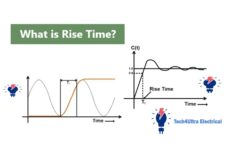
From a waveform perspective, the definition of rise time refers to the time it takes for a signal to transition from its low voltage level to its high voltage level. Specifically, it’s the time the signal takes to move from a small percentage of its final value—typically 10%—to a higher percentage, like 90%.

So when a signal jumps from low to high, it doesn’t do so instantly—it ramps up. That time interval is your rise time.

Graphical representation

If you were to draw this on a graph, you’d see a curve climbing from near-zero up to a peak. Instead of a vertical wall (which would mean instant transition), there’s always a slope. The steeper the slope, the faster the rise time. If it’s slow, that slope becomes a hill—and in high-speed systems, that hill can ruin your signal quality.

Common measurement conventions (10–90 %, 5–95 %, 0–100 %)

Over time, I learned that not all engineers measure rise time the same way. The most common standard is 10–90%, which means the clock starts at 10% of the signal’s final value and stops at 90%. But there are others too—some prefer 5–95%, and purists might go for 0–100% (though that’s less practical).

10–90%: Most commonly used, good balance between precision and simplicity.
5–95%: Used for higher precision measurements.
0–100%: Theoretical ideal, but not very reliable due to noise and overshoot.

Understanding these measurement points is crucial. Trust me, nothing’s more frustrating than comparing rise times from two sources only to realize they used different conventions.

The Physics Behind Rise Time

Signal transition behavior

I used to think an electrical signal just instantly “turned on” like a light switch. But physics had other plans. The truth is, every signal takes time to transition—from low to high, or vice versa. That transition is what defines the rise time, and it’s not just a function of voltage—it’s influenced by physical properties in the circuit.

Signals aren’t magical—they travel through real materials. They face resistance, capacitance, and sometimes reactance. This means they accelerate slowly, like a car from a full stop. That transition curve you see? It’s the signature of your system’s physical limits.

Effect of capacitance and inductance

Here’s where it gets more interesting. The rise time in any system is heavily affected by capacitance and inductance. A capacitor resists change in voltage, and an inductor resists change in current. Together, they introduce lag in how fast a signal can rise.

For example, in a simple RC circuit, the more capacitance you have, the slower the signal rises. It’s like trying to fill a huge water tank with a small pipe. More capacitance = more delay. Inductance adds another twist, especially in high-frequency systems. It can cause ringing or overshoot, which messes up the clean edges of your signal.

Relation to system inertia and delay

Think of rise time as the “inertia” in your system. Just like a physical object doesn’t accelerate instantly due to mass, a signal doesn’t rise instantly due to electrical inertia. That delay is what causes longer rise times. The more your system resists change, the slower the response.

In digital systems, this affects how many bits you can transfer per second. In analog, it affects fidelity. Understanding these delays helped me improve not just performance, but reliability. Once I learned to “read” the physics behind the rise time, troubleshooting circuits became so much easier.

How to Calculate Rise Time

General equation: t_r = t₂ – t₁

The first time I tried to measure rise time, I used this classic equation: t_r = t₂ – t₁. It’s basic but super effective. You just subtract the time the signal hits 10% (t₁) from the time it hits 90% (t₂). That’s your rise time. Simple, right?

This works for most waveforms and gives you a solid starting point before jumping into more advanced formulas. Just make sure your measurements are accurate—use cursors or software markers on an oscilloscope to avoid guessing.

RC circuit: t_r ≈ 2.197 × τ

When dealing with an RC (resistor-capacitor) circuit, the rise time equation gets more interesting. The approximation t_r ≈ 2.197 × τ (where τ = R × C) works great for step responses. I remember testing this in the lab and getting results within 5% of the theoretical value—it felt like magic!

This formula assumes the standard 10–90% range. If your circuit has a high capacitance, expect a slower rise time. Want to speed it up? Reduce the capacitance or resistance, but be mindful of power dissipation.

RL circuit approximation

For RL (resistor-inductor) circuits, it’s a bit different. The rise time isn’t linear because inductors behave like resistors at DC and react to change in current. The formula varies, but an estimate for rise time is often close to t_r ≈ 3 × L/R. That gives you a good starting point if you’re simulating or debugging analog filters.

Gaussian and cascaded systems

When I got deeper into signal processing, I came across Gaussian systems. In these systems, the rise time is related to the bandwidth using an inverse relationship: t_r ≈ 0.35/BW. This is super helpful when you’re dealing with oscilloscope probes, amplifiers, or any system with Gaussian roll-off.

In cascaded systems, rise times add up in quadrature: t_r-total = √(t₁² + t₂² + t₃² + …). I once ignored this in a project and ended up with sluggish performance because each stage added more delay.

Real-world examples with calculations

Here’s a quick one: Suppose you have an RC low-pass filter with R = 1kΩ and C = 100nF. That gives τ = 0.0001 seconds. Multiply by 2.197, and you get t_r ≈ 219.7 μs. You’ll actually see this slope on the oscilloscope—proof that theory meets reality.

Understanding how to use the rise time equation lets you predict behavior before even building a circuit. Trust me, that’s a massive time saver when prototyping or debugging.

Bandwidth and Rise Time Relationship

Explanation of BW × t_r ≈ constant

This is the formula that really opened my eyes: Bandwidth × Rise Time ≈ Constant. I used to think rise time and bandwidth were separate things—until I realized they’re two sides of the same coin. The faster your signal rises, the wider the frequency range needed to represent that rise accurately.

For many systems, especially with Gaussian or first-order low-pass characteristics, the rule of thumb is BW × t_r ≈ 0.35. This approximation helps you estimate either the bandwidth or the rise time if one of them is unknown. It saved me more than once while selecting test equipment or predicting system behavior.

Frequency domain interpretation

Here’s where things click: A fast rise time in the time domain requires higher-frequency components in the frequency domain. That’s because sharp transitions contain a wide range of frequencies. Limit the bandwidth, and you blunt that sharp edge—your square wave turns into a slope.

When designing systems, I always check if the bandwidth is enough to preserve the edges of my signals. If not, the output starts to resemble a sine wave more than a digital pulse, and that’s when errors creep in.

Examples with bandwidth values

Let’s say your oscilloscope probe has a bandwidth of 100 MHz. Using the formula t_r ≈ 0.35 / BW, that gives a rise time of about 3.5 ns. That means you can’t accurately measure rise times faster than that. I learned this the hard way—my probe was limiting the signal I thought I was analyzing.

Another example: if a system has a rise time of 70 ns, then its effective bandwidth is around 5 MHz. It’s a quick check that gives powerful insight, especially when you’re troubleshooting or validating signal quality.

Bottom line: bandwidth and rise time are locked together. If one changes, the other follows. Get to know this relationship well—it’ll become one of your favorite tools in the lab.

Rise Time in Different Systems

RC and RL circuits

My first hands-on experience with rise time was through RC and RL circuits in a university lab. RC circuits are straightforward—the rise time is mostly shaped by the resistor and capacitor. It’s proportional to the RC time constant, which means more capacitance or resistance equals a slower signal response.

For RL circuits, it’s the opposite side of the same coin. Instead of voltage, the inductor limits how fast current can rise. You’ll see rise times stretching with higher inductance. The difference? RC circuits respond to voltage steps, while RL circuits respond to current. But in both cases, the components act like brakes on the transition.

Second-order control systems (underdamped vs overdamped)

Now, second-order systems are where things get nuanced. When I started working with motor controllers, I had to learn fast about underdamped and overdamped behavior. An underdamped system overshoots its final value and oscillates before settling—its rise time is fast, but it comes with a tradeoff: instability.

In an overdamped system, there’s no overshoot—it’s a slow, steady climb to the final value. That sounds nice, but it means longer rise times. Somewhere in between is the critically damped system: no overshoot, minimal delay. That’s the sweet spot in many practical designs, like servos and sensor feedback systems.

Gaussian and critically damped systems

In high-speed digital circuits, Gaussian responses are ideal because they’re smooth and predictable. They avoid ringing and overshoot while keeping rise time sharp enough for reliable logic transitions. A Gaussian system has a rise time directly related to its bandwidth (t_r ≈ 0.35/BW), which makes it easy to model.

Critically damped systems, on the other hand, are common in control engineering. They offer the best balance between speed and stability. I’ve used this damping model in robotic arms where any overshoot could cause mechanical issues.

Practical use-case comparisons

Let’s compare: In audio circuits, long rise times are acceptable because human ears can’t detect fast voltage changes. But in microcontrollers switching at 100 MHz, a long rise time might corrupt data or cause timing errors. That’s why rise time matters so much—it’s context-specific.

RC circuits: Predictable but slow transitions—great for filters.
Underdamped systems: Fast but risky—good for speed-critical applications.
Gaussian systems: Balanced and clean—excellent for signal integrity.
Critically damped systems: Best for stability without sacrificing too much speed.

Learning to choose the right rise time profile for each system is part art, part science. But once you get the hang of it, it’s one of the most powerful tools in your design toolbox.

Common Mistakes and Misconceptions

Confusing rise time with delay or settling time

Early on, I made the classic mistake: thinking rise time was just another name for delay. Nope. Rise time is the time it takes for a signal to go from 10% to 90% of its final value—not the time it takes to start moving or to fully settle. That’s where delay and settling time come in, and they’re very different.

Delay is when the signal starts to respond. Settling time is how long it takes to reach and stay within a tolerance band around the final value. But rise time? It’s all about that transition zone, and mixing them up can lead to design errors and bad diagnostics.

Incorrect use of measurement thresholds

Another trap I fell into was using the wrong thresholds for measuring rise time. If you’re using 5–95% in one part of your project and 10–90% in another, your numbers won’t match up. That tiny difference throws off bandwidth estimates and system comparisons. Be consistent—it makes your data meaningful.

Misinterpretation in non-linear systems

Non-linear systems are a whole different beast. I once tried to measure rise time on a signal that wasn’t even monotonic—it overshot, oscillated, and didn’t settle cleanly. That’s when I learned: in non-linear or noisy systems, you can’t just apply standard formulas blindly. Always interpret rise time in context, or you might be reading noise instead of performance.

Applications of Rise Time

High-speed digital circuits

If you’re designing high-speed digital circuits, rise time becomes one of your most critical parameters. I once worked on a microcontroller interface running at 200 MHz—every nanosecond counted. If the rise time was too slow, the logic levels didn’t reach their thresholds in time, causing bit errors and timing violations. Fast rise times ensure sharp edges and reliable switching, especially when clock and data signals must sync precisely.

Analog signal filtering

In analog circuits, like audio filters or sensor signal conditioners, rise time tells you how quickly the system can respond to a change in input. I found that adjusting filter components directly impacted rise time—too slow, and your output lags behind the real signal. Too fast, and you start passing noise. So tuning rise time in filters is about balance: fast enough for responsiveness, slow enough for stability.

Control systems tuning

When tuning PID controllers or designing automation systems, rise time is one of the go-to metrics. A short rise time means your system reacts quickly—but it might overshoot or oscillate. A long rise time makes things sluggish but stable. I’ve spent hours tuning these settings, and it always comes down to what’s more important: speed or smoothness.

Signal integrity in communication

Rise time directly affects signal integrity in data communication systems. Ethernet, USB, and even HDMI all depend on clean, fast signal transitions. I learned this firsthand debugging a USB interface where long rise times caused intersymbol interference. Improving the driver’s slew rate helped restore clean communication. In short, managing rise time keeps your signals sharp and your data reliable.

Advanced Topics: Rise Time in Cascaded Systems

Impact of multiple stages

When I first started designing multi-stage amplifiers, I assumed each stage would simply pass the signal along. What I didn’t realize was that each stage added a bit of delay—and that meant longer rise time. In cascaded systems, these delays stack up in a way that can cripple performance if not managed carefully.

Even if each individual stage has a decent rise time, combining them without considering cumulative effects leads to sluggish transitions. I learned quickly that a system is only as fast as its slowest stage—or the square root of the sum of their squared rise times, to be more precise.

Calculating effective rise time

There’s a go-to formula for this: t_r-total = √(t₁² + t₂² + t₃² + …). This approach assumes each stage behaves like a Gaussian or low-pass filter. It’s not perfect, but it gives a solid estimate of the system’s overall rise time.

For example, if three stages have rise times of 5 ns, 7 ns, and 10 ns, the total rise time is about √(25 + 49 + 100) ≈ 13.9 ns. That’s a big jump, and if you’re targeting sub-10 ns transitions, your design won’t meet spec unless you improve one or more stages.

Limiting factors and design considerations

Things get trickier when parasitics and layout come into play. Long traces, bad impedance matching, and connector losses can add hidden rise time penalties. I once worked on a design that passed simulations but failed on the bench—all due to trace inductance I hadn’t accounted for.

When optimizing rise time in cascaded systems, I now look at:

Bandwidth consistency across stages
Parasitic capacitance and inductance
Proper termination and impedance control
Minimizing unnecessary filters or slow buffers

Understanding how rise time grows across a chain of stages can be the key to hitting performance targets—especially in fast, timing-critical applications like ADC front ends or RF paths.

Watch Also: Low Voltage Switchgear: Types, Components, and Uses

Tools and Techniques for Measuring Rise Time

Using an oscilloscope

The first time I measured rise time, I used an entry-level oscilloscope—and it taught me a lot. Oscilloscopes are the go-to tool for visualizing signal transitions. You simply hook up your probe, set the voltage and time divisions, and zoom in on the rising edge of your signal. Use the cursor or measurement tools to mark the 10% and 90% levels, and you’ll get a pretty accurate rise time reading.

Just make sure your oscilloscope has sufficient bandwidth. A scope with a 20 MHz bandwidth won’t give you a proper view of a 2 ns rise time. I learned to match my measurement tool to my signal speed—otherwise, you’re not measuring the signal, you’re measuring the scope’s limits.

Software simulation tools

Before even touching the bench, I use simulation tools like LTspice or Multisim to predict rise time behavior. They let you test various circuit configs without burning components. While not always perfect, they give valuable insights—especially when dealing with filters or multi-stage systems.

Accuracy tips and setup advice

To get precise rise time readings, follow a few simple rules:

Use the shortest possible ground lead on your oscilloscope probe
Match probe bandwidth to your signal
Use differential probes for high-speed, low-noise measurements
Avoid triggering errors by setting your level near 50% of the waveform height

Trust me, measuring rise time isn’t hard—but doing it right makes all the difference.

Conclusion

Main formulas recap

Let’s wrap this up with the key formulas you’ll want to keep in your toolkit:

t_r = t₂ – t₁: Basic rise time calculation (10–90% levels)
t_r ≈ 2.197 × τ: For RC circuits (where τ = R × C)
t_r ≈ 3 × L / R: Approximate rise time in RL circuits
t_r ≈ 0.35 / BW: Gaussian systems and bandwidth estimation
t_r-total = √(t₁² + t₂² + …): Effective rise time in cascaded systems

When and how to use rise time analysis

Use rise time analysis anytime speed, accuracy, or signal clarity matter—whether you’re debugging a noisy microcontroller line or tuning a precision control loop. It’s a diagnostic, a design guide, and a performance benchmark all in one. Mastering it means you’re not just building circuits—you’re engineering systems that actually work right, fast, and reliably.

Keep these insights handy. The next time someone asks “what’s the rise time?”—you won’t just answer. You’ll explain it like a pro.

FAQs

What is the equation for rise time?

The most common rise time equation is t_r = t₂ – t₁, where t₂ is the time the signal reaches 90% of its final value, and t₁ is the time it reaches 10%. This basic definition applies to digital and analog signals alike. In RC circuits, you can also use t_r ≈ 2.197 × τ, where τ is the time constant (R × C).

What is the rise time method?

The rise time method involves measuring how long it takes a signal to go from a low voltage (typically 10%) to a high voltage (usually 90%) of its final value. It’s commonly used to evaluate the speed of transitions in electronics, signal processing, and communication systems. Engineers use this method to diagnose performance issues and validate signal integrity.

What is the calculation of rise?

To calculate rise time, simply subtract the time at 10% from the time at 90% of the signal’s final amplitude. Example: If your signal rises from 10% at 3 ns to 90% at 8 ns, the rise time is 5 ns. In systems like RC filters, rise time is calculated based on component values using known formulas.

How do you measure rise time?

Use an oscilloscope to measure rise time. Set up the probe correctly, display the waveform, and use the scope’s cursor or built-in measurement tools to mark the 10% and 90% amplitude levels. The time difference between these two points is your rise time. For precision, make sure your scope has enough bandwidth to capture fast transitions accurately.

Contents