How to Calculate DC Gain of a Transfer Function (With Examples)

Struggling to understand what DC gain really means or how the transfer function shapes system behavior? You’re not alone. Many students and even junior engineers treat these terms as abstract math, missing their real-world impact. In this article on the Tech4Ultra Electrical website, I’ll break down these concepts in a clear, practical way—so by the end, you’ll not only understand them, but actually know how to use them with confidence.

What is a Transfer Function?

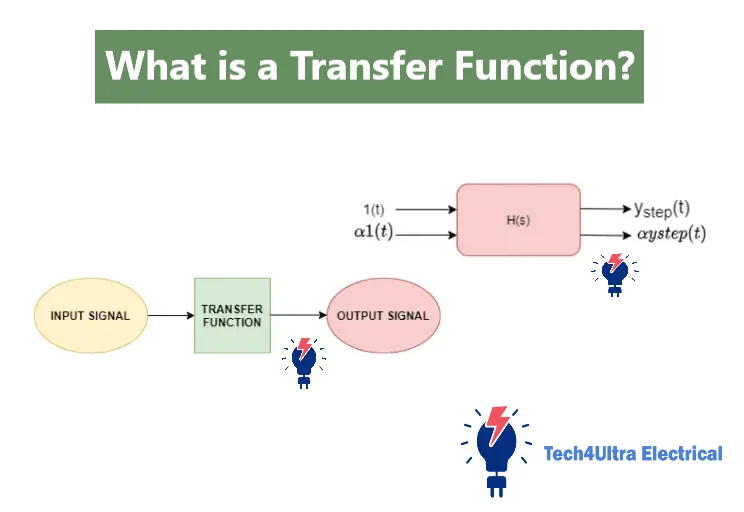
Imagine trying to understand how a car responds when you press the gas pedal. You apply an input (pressing the pedal), and the car responds with an output (speeding up). In engineering, we describe this input-output relationship using something called a transfer function. At its core, a transfer function is a mathematical formula—usually expressed in terms of Laplace variable s—that shows how the output of a system responds to any given input.

The beauty of a transfer function is that it simplifies complex systems. Rather than dealing with multiple equations or physical parts, we use one function to represent the entire system’s behavior. It’s like turning a messy, tangled set of wires into a single clean cable.

Role in System Modeling

In control systems and signal processing, the transfer function is crucial. It lets engineers model and predict how a system behaves without physically building it. Want to see if a drone stays stable during flight or if an amplifier distorts audio signals? Use the transfer function.

Examples of Real-World Systems

• In an audio equalizer, the transfer function helps shape sound frequencies.
• In robotics, it models how a motor reacts to voltage changes.
• In finance, it can even represent how investments respond to economic input.

Read Also: Rise Time: Definition, Formula, and Practical Examples

Definition of DC Gain in Control Systems

Formal Definition Using Ratio of Steady-State Output to Input

In control systems, DC gain is a key metric that tells us how much a system amplifies or attenuates a signal when the input is constant. More formally, it’s defined as the ratio of the steady-state output to the steady-state input when the input is a step function. This gives engineers a simple but powerful way to measure how a system behaves in the long run.

If you apply a constant input—say a fixed voltage or position—and wait long enough, the system will eventually settle. The value it settles at is called the steady-state output. Divide that by the original steady-state input, and you’ve got the DC gain.

Integration with Laplace Transform Concepts

To compute DC gain mathematically, we turn to the transfer function in the Laplace domain. Here’s the trick: substitute s = 0 into the transfer function. Why? Because s = 0 corresponds to a constant input in Laplace transform theory—essentially a signal that doesn’t change over time.

So, the DC gain equals the value of the transfer function when s = 0. This is often written as G(0) for systems with a transfer function G(s). It’s a quick way to understand the long-term amplification or attenuation behavior of any linear time-invariant (LTI) system.

Watch Also: High Voltage Switchgear: Types, Components, and Safety

Mathematical Derivation and Formula

Detailed Derivation: lim_s→0 G(s)

The DC gain of a system is derived using the transfer function G(s). The most direct way to find it is to evaluate the transfer function at s = 0. Mathematically, this is written as:

DC Gain = lim_s→0 G(s)

This works because s = 0 in the Laplace domain corresponds to a constant input in the time domain. When you plug in s = 0 into G(s), you’re essentially seeing the system’s response to a step input after all transients have died out.

Explanation Using Final Value Theorem

The final value theorem helps justify this mathematically. It states:

lim_t→∞ y(t) = lim_s→0 sY(s)

Assuming a unit step input (1/s), we know Y(s) = G(s) * 1/s. So:

lim_t→∞ y(t) = lim_s→0 s * [G(s)/s] = G(0)

Hence, the final value of the output—our steady-state output—is exactly the DC gain of the system.

Contextual Example with Equations

Take a basic system with a transfer function G(s) = 5 / (s + 2). To find the DC gain:

lim_s→0 G(s) = 5 / (0 + 2) = 2.5

This tells us the system will settle at 2.5 times the input value when a constant input is applied—a clear, practical measure of long-term system behavior.

How to Find DC Gain – Step-by-Step Method

Easy-to-Follow Steps with Inline Examples

If you’re wondering how to find the DC gain of a transfer function, don’t worry—it’s simpler than it looks. Follow these steps:

1. Write the transfer function G(s) – Start by expressing your system’s behavior in the Laplace domain.
2. Substitute s = 0 – Evaluate G(s) at s = 0 to find the DC gain.
3. Simplify the result – Perform the necessary algebra to get a numerical answer.

Example: Say G(s) = (3s + 6) / (s² + 4s + 5). Plug in s = 0:

G(0) = 6 / 5 = 1.2

That’s your DC gain—simple and fast.

Different Approaches for Open-Loop and Closed-Loop Systems

The method varies slightly depending on whether the system is open-loop or closed-loop.

• Open-loop system: Just apply the basic steps above directly on the transfer function G(s).
• Closed-loop system: Use the closed-loop transfer function:
  T(s) = G(s) / (1 + G(s)H(s))
  Then evaluate T(s) at s = 0 to find the DC gain.

Example: If G(s) = 10 / (s + 5) and H(s) = 1, then:

T(s) = 10 / (s + 15), and T(0) = 10 / 15 = 0.666

That’s how you find the DC gain for closed-loop systems.

Worked Examples

Example 1: First-Order System

Let’s start simple with a first-order system: G(s) = 4 / (s + 2)

To find the DC gain, evaluate G(s) at s = 0:

G(0) = 4 / (0 + 2) = 2

This means the system’s steady-state output will be twice the steady-state input. The DC gain here is 2, which represents the system’s static gain. So, a constant input of 1 results in an output of 2 in steady state.

Example 2: Second-Order System

Consider this transfer function: G(s) = 10 / (s² + 3s + 10)

To find the DC gain:

G(0) = 10 / (0 + 0 + 10) = 1

In this case, the DC gain is 1. This means there is no amplification or attenuation of a constant input. The static gain interpretation is straightforward: a unit input results in a unit output.

Example 3: Feedback System with H(s) ≠ 1

Now let’s try a more realistic scenario with feedback: G(s) = 5 / (s + 5) and H(s) = 2

First, derive the closed-loop transfer function:

T(s) = G(s) / (1 + G(s)H(s)) = [5 / (s + 5)] / [1 + (5 * 2) / (s + 5)]

Simplifying:

T(s) = 5 / (s + 15)

Now plug in s = 0:

T(0) = 5 / 15 = 0.333

This tells us the DC gain is 0.333, meaning the system reduces the steady-state input to one-third of its value in output. The static gain here shows the effect of strong feedback reducing system sensitivity.

Each of these examples highlights a key insight: DC gain provides a quick way to understand a system’s long-term behavior. Whether amplifying, preserving, or reducing the input, this value defines the final relationship between input and output.

Understanding DC Gain in Frequency Domain

Link to Low-Frequency Behavior and Bode Plots

When analyzing systems in the frequency domain, the DC gain tells us how the system behaves at very low frequencies—specifically as frequency approaches zero. In other words, it represents the low-frequency gain of the system. This is especially important when you’re interpreting a Bode plot.

On a Bode plot, the DC gain corresponds to the magnitude at 0 rad/s. It sets the baseline for how the system responds to steady or slowly changing signals. For instance, a Bode magnitude plot starting at 20 dB means the DC gain is 10, since 20 dB = 20log₁₀(10).

This low-frequency response—also called the small-signal gain—is a critical indicator of how the system reacts to small, slowly varying inputs. It helps in understanding behavior before higher-frequency dynamics take over, such as phase shifts or resonance peaks.

In practical applications like audio systems, motor controllers, or sensor circuits, knowing the low-frequency gain helps ensure the system performs accurately and stably under normal operating conditions.

So whether you’re tuning filters or assessing amplifier behavior, the DC gain and its interpretation on a Bode plot give you direct insight into the system’s long-term or baseline performance.

Watch Also: Star Delta Starter: Comprehensive Guide to Working, Circuits, and Applications

Applications and Importance of DC Gain

Use in Controller Design, Performance Tuning

In any control system, understanding the DC gain is crucial for designing effective controllers and tuning performance. A controller adjusts the input to keep the output as close as possible to a desired value. Knowing the DC gain helps you predict the final output response to a step input, which is key when minimizing steady-state error.

For example, in proportional control, increasing the proportional gain changes the DC gain of the loop, improving accuracy but possibly affecting system speed or stability. It’s a balancing act, and DC gain gives you the data to make those trade-offs wisely.

Impact on Stability and System Response

While DC gain primarily reflects steady-state behavior, it indirectly influences system dynamics. Adjusting it may shift the poles and zeros of the system, affecting response time, overshoot, and even the damping ratio. This means tuning DC gain isn’t just about accuracy—it’s also about achieving a smooth, stable system response.

That’s why engineers never ignore DC gain. It’s a small value with a big role in shaping how your control system behaves both statically and dynamically.

Common Mistakes and Misconceptions

DC Gain ≠ Gain at All Frequencies

One of the most common mistakes is assuming that DC gain applies across all frequencies. That’s simply not true. DC gain only reflects system behavior at s = 0, which means it shows the response to a constant input. It says nothing about how the system reacts to fast-changing or oscillating signals.

Clarifying Confusion in Higher-Order Systems

In higher-order systems, people often misread the DC gain due to complex poles and zeros. They might plug in s = 0 without simplifying the transfer function first, leading to incorrect results. Also, feedback loops with non-unity feedback (H(s) ≠ 1) can further obscure what the DC gain truly represents.

To avoid these pitfalls, always analyze the structure of the system and verify what part of the transfer function you’re evaluating. Remember: DC gain is just one snapshot of the system—valuable, but not the full picture.

Conclusion

Recap of Main Concepts and Formulas

To wrap up: the DC gain is the system’s output-to-input ratio at steady state, calculated by evaluating the transfer function at s = 0. The formula:

DC Gain = lim_s→0 G(s)

Use the final value theorem to justify this in Laplace-based systems and always simplify your transfer function before plugging in s = 0.

Key Things to Remember for Exams or Practical Use

• DC gain only applies to constant or low-frequency inputs—not all frequencies.
• Always account for feedback paths when calculating DC gain in closed-loop systems.
• In Bode plots, DC gain appears at 0 rad/s and reflects the system’s low-frequency gain.
• Understand the difference between DC gain and overall system gain—it can save you marks on exams and time in real-world debugging.

Keep these tips in mind, and you’ll approach any control system question with confidence.

FAQ

What is DC gain in layman’s terms?

Think of DC gain as how much output you get when you feed a system a steady, unchanging input. If you give your system a constant signal—like flipping a light switch on—and the output responds by doubling that signal, the DC gain is 2. It’s like asking: “For every 1 unit I put in, how many units come out once everything settles?”

How do I know if my DC gain is too high or low?

It depends on what your system needs to do. A DC gain that’s too high might mean your system overreacts to inputs—potentially causing instability or overshoot. A DC gain that’s too low might lead to sluggish performance or large steady-state errors. In controller tuning, you often adjust DC gain to balance responsiveness with accuracy.

Does DC gain affect transient response?

Not directly. DC gain tells you about the system’s final, steady behavior—not how it gets there. But tweaking DC gain can shift your system’s poles and zeros, which in turn affects things like overshoot, rise time, and settling time. So while DC gain is about the end result, it can influence the journey indirectly through system dynamics.

Understanding these subtle effects is what separates good control engineers from great ones.

What is the gain of a control system example?

In a simple control system like G(s) = 10 / (s + 2), the gain represents how much the system amplifies the input. At s = 0, the gain is 10 / 2 = 5. This means if you apply a steady input of 1, the output will settle at 5. This value is called the DC gain.

What is the DC gain?

DC gain is the ratio of a system’s steady-state output to its steady-state input when the input is constant (DC signal). Mathematically, it’s G(s) evaluated at s = 0. It shows how a system behaves in the long term when no change is happening.

What is the DC gain of a filter circuit that has the given transfer function?

To find the DC gain of a filter, substitute s = 0 into its transfer function G(s). For example, if G(s) = 1 / (s + 10), then G(0) = 1 / 10 = 0.1. This means the filter passes only 10% of the steady (DC) input through to the output.

What is the formula for DC gain of open loop?

The formula is simple: DC gain = G(0), where G(s) is the open-loop transfer function. Just evaluate it at s = 0. This gives you the gain of the system in response to a constant input, before any feedback is applied.