Contents
Have you ever spent hours designing a control system only to realize it doesn’t perform as accurately as expected? The culprit might be something often overlooked: steady state error. In this article on the Tech4Ultra Electrical website, you’ll learn what steady state error really means, how it behaves in unity feedback and non-unity feedback systems, and why mastering this concept is key to building more precise and reliable control systems. Stick around to gain practical insights that could completely change how you approach your system design.
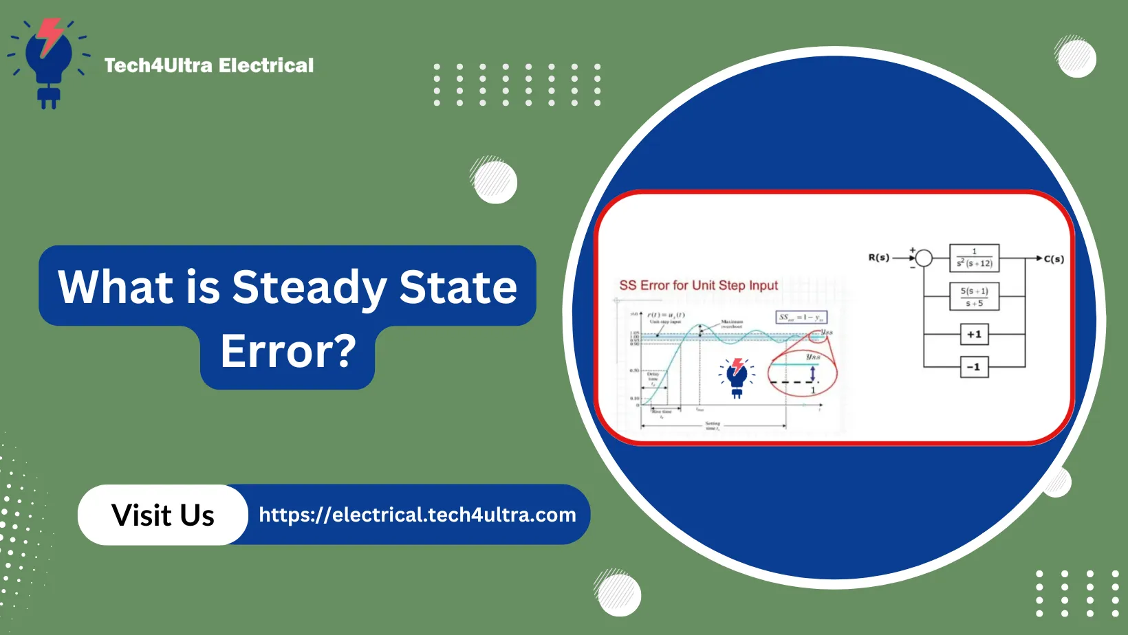
What Is Steady State Error (SSE)?
Steady state error (SSE) refers to the difference between a system’s desired output and its actual output after it has settled and reached steady conditions. In simpler terms, it’s the small amount of error that remains even after the system has had enough time to respond to an input. It’s like asking a robot arm to move to a specific point and it gets close, but not exactly there—this small miss is the steady state error.
Mathematically, SSE can be calculated using the final value theorem:
SSE = limt→∞ e(t) = lims→0 s * E(s)
Where e(t) is the error signal over time, and E(s) is its Laplace transform. This formula helps engineers determine how accurate their control system is in reaching the desired output.
Why Is SSE Important?
In any control system, minimizing steady state error is crucial for accuracy and performance. Whether you’re building a temperature control unit or a robotic arm, you want the system to respond correctly to commands. High SSE can mean poor performance, wasted energy, or even system instability.
Real-World Relevance
Steady state error isn’t just theory—it has real-world consequences. In industrial automation, if a robotic arm misses its target by even a few millimeters due to SSE, it could result in defective products. In robotics, accurate positioning is vital, and even small errors can affect functionality. That’s why understanding SSE is a must for engineers in modern system design.
Read Also: How to Calculate DC Gain of a Transfer Function (With Examples)
Fundamental Concepts
Steady State vs. Transient Response
When analyzing a control system, it’s important to distinguish between two key behaviors: the transient response and the steady state response. The transient response is what happens immediately after a system experiences a change in input—this includes overshoots, oscillations, and rapid changes. It’s like when you suddenly turn your car’s steering wheel—the quick wobbles that follow are the transient phase.
The steady state response is what the system settles into after all those wobbles disappear. It’s the long-term behavior of the system, and it’s where we measure the steady state error. This is the part that tells us how close the system gets to the desired outcome once all the initial chaos calms down.
Actuating Signal vs. System Output
In a feedback system, the actuating signal is the difference between the input signal (what you want the system to do) and the feedback signal (what the system is actually doing). This error signal is what drives the controller to act. The system output, on the other hand, is the actual behavior or response of the system.
In a unity feedback system, the output is directly compared with the input to generate this error. In non-unity feedback systems, there might be modifications to the feedback signal before it’s compared to the input, which affects how SSE is analyzed.
Conditions for SSE Analysis
Before you can analyze steady state error, there’s one major requirement: the system must be closed-loop stable. This means that all the poles of the system’s transfer function should lie in the left-half of the complex plane (for continuous systems). Without stability, the output never settles, and calculating SSE becomes meaningless.
So, make sure your system is stable before even thinking about SSE.
System Types and Error Constants
System Classification: Type 0, Type 1, Type 2
To understand steady state error behavior, we first classify control systems based on the number of integrators (poles at the origin) in the open-loop transfer function. This classification helps predict how the system will respond to different inputs:
- Type 0: No poles at the origin
- Type 1: One pole at the origin
- Type 2: Two poles at the origin
Each type behaves differently when subjected to inputs like step, ramp, or parabolic signals, and directly affects the steady state error of the system.
Error Constants: Kp, Kv, Ka
To quantify SSE, we use error constants—these are standard values that predict how a system type handles specific input signals.
- Kp (Position error constant): Measures SSE for a step input
- Kv (Velocity error constant): Measures SSE for a ramp input
- Ka (Acceleration error constant): Measures SSE for a parabolic input
These constants are computed using the open-loop transfer function G(s) and the feedback transfer function H(s). For unity feedback systems, SSE formulas become more straightforward.
How System Type Affects SSE
As the system type increases, its ability to track more complex input signals improves. For instance, a Type 0 system can only track a step input with a finite error. A Type 1 system completely eliminates error for a step input and reduces error for ramp inputs. A Type 2 system can handle both step and ramp inputs with zero error and even reduces error for parabolic inputs.
Here’s a practical interpretation:
| System Type | Step Input | Ramp Input | Parabolic Input |
|---|---|---|---|
| Type 0 | Finite SSE (1/(1+Kp)) | Infinite SSE | Infinite SSE |
| Type 1 | Zero SSE | Finite SSE (1/Kv) | Infinite SSE |
| Type 2 | Zero SSE | Zero SSE | Finite SSE (1/Ka) |
Understanding this table gives you the tools to design systems that meet your precision goals. Whether working on non-unity feedback loops or real-world robotic controls, system type is a critical design decision.
SSE Analysis Using Final Value Theorem
What is the Final Value Theorem?
The Final Value Theorem is a powerful tool in control systems for analyzing the steady state error. It allows us to calculate the final value of a time-domain function using its Laplace transform, assuming the system is stable.
The formula is simple:
limt→∞ f(t) = lims→0 s * F(s)
Where F(s) is the Laplace transform of f(t). For SSE, we apply this to the error signal E(s) to compute the error at steady state:
SSE = lims→0 s * E(s)
Error Expressions for Common Inputs
To calculate SSE, we use a standard block diagram where the system has an open-loop transfer function G(s) and a feedback function H(s). For unity feedback (H(s) = 1), the closed-loop transfer function becomes:
T(s) = G(s) / (1 + G(s))
And the error function is:
E(s) = R(s) / (1 + G(s))
1. Step Input (R(s) = 1/s)
SSE = lims→0 s * (1/s) * (1 / (1 + G(s))) = 1 / (1 + Kp)
2. Ramp Input (R(s) = 1/s²)
SSE = lims→0 s * (1/s²) * (1 / (1 + G(s))) = 1 / Kv
3. Parabolic Input (R(s) = 1/s³)
SSE = lims→0 s * (1/s³) * (1 / (1 + G(s))) = 1 / Ka
Block Diagram Interpretation
In most practical systems, especially with non-unity feedback, the error function becomes more complex, as H(s) is no longer 1. In such cases, the modified error becomes:
E(s) = R(s) – Y(s) = R(s) – G(s)H(s) / (1 + G(s)H(s)) * R(s)
Analyzing these expressions allows engineers to determine how system design choices affect long-term performance.
Unity vs Non‑Unity Feedback Systems
Definitions of Feedback Configurations
In control systems, the structure of the feedback loop plays a critical role in system behavior and steady state error performance.
A unity feedback system is one where the feedback signal is directly equal to the output. This means the feedback path contains no additional elements, and H(s) = 1. These systems are easier to analyze and are often used in theoretical studies.
In contrast, a non-unity feedback system includes elements in the feedback path—like sensors or filters—resulting in H(s) ≠ 1. These are more realistic in real-world systems, where measurements and actuators often modify the feedback signal.
Transforming Non-Unity into Unity Feedback
To analyze a non-unity feedback system using simpler unity feedback methods, we can convert it into an equivalent unity feedback structure. This involves redefining the open-loop transfer function.
If you have a system where the original configuration is:
Y(s) = G(s) * [R(s) – H(s) * Y(s)]
You can manipulate the equation into a form that resembles:
Y(s)/R(s) = Geq(s) / (1 + Geq(s))
Where: Geq(s) = G(s) / (1 + G(s)[H(s) – 1])
This “equivalent” system allows us to apply familiar steady state error formulas using the final value theorem.
SSE Formulas and Key Differences
For a unity feedback system:
SSE = lims→0 s * [R(s)/(1 + G(s))]
But for a non-unity feedback system:
SSE = lims→0 s * [R(s) – G(s)H(s) / (1 + G(s)H(s)) * R(s)]
This expression requires extra care, especially when H(s) introduces dynamics like time delays or filtering.
While unity feedback gives clean, straightforward analysis, non-unity feedback reflects more realistic systems, demanding deeper understanding of the feedback path and how it influences overall performance.
Practical Examples with Calculations
Example 1: Unity Feedback, Type 0 System
Consider a control system with open-loop transfer function: G(s) = 5 / (s + 2). Since there are no poles at the origin, this is a Type 0 system.
Input: Step (R(s) = 1/s)
For unity feedback, the error signal is:
E(s) = R(s) / (1 + G(s)) = (1/s) / (1 + 5 / (s + 2)) = (1/s) * (s + 2) / (s + 7)
Using the final value theorem:
SSE = lims→0 s * E(s) = lims→0 s * (1/s) * (s + 2)/(s + 7) = (2/7) ≈ 0.286
Example 2: Non-Unity Feedback, Type 1 System
Now consider: G(s) = 10 / (s(s + 3)), and feedback function H(s) = 0.5. This system has one pole at the origin → Type 1.
Input: Ramp (R(s) = 1/s²)
First, find the closed-loop transfer function:
T(s) = G(s)H(s) / (1 + G(s)H(s)) = [10 * 0.5 / (s(s + 3))] / [1 + 10 * 0.5 / (s(s + 3))]
Simplify: T(s) = 5 / (s² + 3s + 5)
Error signal: E(s) = R(s) – T(s) * R(s) = R(s)[1 – T(s)] = (1/s²) * [1 – 5 / (s² + 3s + 5)]
Now apply the final value theorem:
SSE = lims→0 s * E(s) = lims→0 s * (1/s²) * [(s² + 3s + 5 – 5)/(s² + 3s + 5)] = lims→0 (1/s) * (s² + 3s)/(s² + 3s + 5)
As s → 0: SSE = (0 + 0) / 5 = 0
SSE = 0 (Perfect tracking for ramp input)
Comparison
- Unity feedback, Type 0 system: SSE = 0.286 for step input
- Non-unity feedback, Type 1 system: SSE = 0 for ramp input
This shows how increasing system type and designing smart feedback paths greatly improve steady state error performance.
Techniques to Reduce Steady State Error
Using PID Controllers
One of the most effective ways to reduce steady state error is by using PID controllers. These controllers adjust the control signal based on three components:
- Proportional (P): Reduces SSE by increasing the system’s sensitivity to error. The higher the proportional gain, the faster the system responds, but it can cause overshoot.
- Integral (I): Eliminates SSE by summing the error over time. This forces the system to drive the long-term error to zero, making it ideal for Type 0 or Type 1 systems.
- Derivative (D): Doesn’t directly reduce SSE but helps improve system stability and reduce overshoot by reacting to the rate of error change.
Combining these three effects allows for a powerful control strategy that balances error correction with smooth system behavior.
Adding Integrators in System Design
By design, adding an integrator (a pole at the origin) increases the system type. This significantly reduces SSE for more complex inputs. For example:
- Adding one integrator to a Type 0 system makes it Type 1, eliminating SSE for step inputs.
- Adding a second integrator creates a Type 2 system, which eliminates SSE for ramp inputs as well.
This method is especially useful in unity feedback configurations but also applies to non-unity feedback with proper design adjustments.
Adjusting Gain and Controller Tuning
Increasing the gain K in the open-loop transfer function G(s) directly affects the error constants (Kp, Kv, Ka). Higher gain reduces SSE:
- SSE = 1/(1 + Kp) for step input → higher Kp means lower SSE.
- SSE = 1/Kv for ramp input → higher Kv means lower SSE.
But too much gain can lead to instability or excessive overshoot. That’s why gain tuning needs to be balanced carefully.
Tradeoffs with Transient Performance
Reducing steady state error often comes with tradeoffs. Adding integrators or increasing gain may:
- Slow down system response
- Increase overshoot
- Cause oscillations or instability if not tuned properly
The key is to find a sweet spot where SSE is minimized without sacrificing too much of the transient behavior. Smart controller tuning, especially in PID-based systems, helps achieve this balance.
Watch Also: Rise Time: Definition, Formula, and Practical Examples
Real-World Applications and Case Studies
Applications in DC Motor Control and Temperature Regulation
Steady state error plays a critical role in many real-world systems where precision is essential. In DC motor control, for instance, SSE determines how accurately the motor reaches and maintains the desired speed or position. A high SSE in a robotic arm could mean missing a pick-up point by millimeters—potentially causing costly production errors.
In temperature regulation systems, like those used in industrial ovens or HVAC units, SSE reflects the gap between the setpoint and the actual temperature. Even a small error could lead to energy inefficiency or product inconsistency in food and pharmaceutical processing.
How Industries Measure and Minimize SSE
Industries measure SSE using sensors and feedback mechanisms that continuously monitor the system’s output. For example, in non-unity feedback systems, smart sensors preprocess signals before feeding them back into the controller. Advanced analytics then compare real-time data against the desired outcome.
To minimize SSE, industries deploy PID controllers, add integrators, or fine-tune control gains. Regular calibration and performance audits also help keep SSE within acceptable bounds.
Role in High-Precision Automation
In sectors like semiconductor manufacturing, aerospace, or 3D printing, even micro-level errors are unacceptable. High-precision automation systems rely on ultra-low SSE for consistent and repeatable output. These systems often use Type 2 control systems with multiple integrators and tightly tuned feedback loops.
Reducing steady state error here is not just about performance—it’s about safety, quality, and meeting strict regulatory standards. That’s why understanding SSE isn’t just theory—it’s the heartbeat of reliable, intelligent automation.
Conclusion
Steady state error may seem like a small detail, but its impact on system performance is massive. Whether in a unity feedback loop or a complex non-unity feedback system, understanding how SSE behaves helps you design smarter, more reliable control systems.
The type of system, the input signal, and the feedback configuration all influence SSE. By adding integrators, tuning gains, or using PID controllers, you can significantly reduce or even eliminate SSE in practical applications.
If you’re serious about control design—whether it’s for robotics, industrial automation, or precision electronics—take the time to explore advanced techniques. Dive deeper into controller tuning, system type analysis, and optimization methods. Reducing steady state error isn’t just about numbers—it’s about delivering performance that users can trust.
FAQs
What happens if the system is unstable?
If a control system is unstable, the concept of steady state error becomes meaningless. That’s because the system output never settles—it keeps growing or oscillating indefinitely. The final value theorem, which we use to calculate SSE, only applies to stable systems. So before calculating SSE, always check for closed-loop stability.
Can SSE ever be zero?
Yes, steady state error can be zero—but only under specific conditions. If you use a properly tuned PID controller or design a system with a high enough type (e.g., Type 1 for step input, Type 2 for ramp input), the SSE can be reduced to zero. However, perfect zero error usually requires ideal conditions with no disturbances or noise.
Does noise affect SSE?
Absolutely. While SSE is calculated for ideal inputs, real-world systems deal with noise from sensors, actuators, or the environment. This noise can affect how accurately the system tracks the input and can make it seem like there’s a steady error when it’s actually signal distortion. Filtering or designing noise-tolerant feedback systems can help minimize this issue.
What is the steady-state error formula?
The steady-state error (SSE) formula depends on the type of input and the system’s configuration. For unity feedback systems, the general formula using the final value theorem is:
SSE = lims→0 s * E(s) where E(s) = R(s) / (1 + G(s))
For step input: SSE = 1 / (1 + Kp) For ramp input: SSE = 1 / Kv For parabolic input: SSE = 1 / Ka
What is a steady-state gain?
The steady-state gain is the value a system’s output reaches after all transients have settled, in response to a constant input. Mathematically, it’s:
K = lims→0 G(s)
It tells you how much of the input signal is passed through the system at equilibrium. A higher steady-state gain generally means a smaller SSE.
What is the steady-state value?
The steady-state value is the final value the output of a control system reaches as time approaches infinity. It reflects the system’s long-term behavior once it stops changing. It’s found using:
limt→∞ y(t) = lims→0 s * Y(s)
How to calculate steady-state values?
To calculate the steady-state value, follow these steps:
- Find the Laplace transform of the output, Y(s).
- Multiply it by s.
- Take the limit as s → 0.
This method assumes the system is stable and that all transients have decayed.
4 thoughts on “Motor Protection Guide: Types, Devices, Faults & NEC Selection Tips”